
Ambiguity Function
How well can a radar distinguish two targets when they have different ranges and velocities? An important tool for answering this question is the ambiguity function (AF). It shows how the output signal of a matched filter depends on signal propagation delay and Doppler frequency. This makes it possible to evaluate how well a particular radar waveform is suited to its intended application.
The ambiguity function is a two-dimensional function χ(τ, fD). Here, τ describes the time shift, while fD represents the Doppler frequency of the signal under consideration. The function describes the response of a matched filter (MF) to time-shifted and Doppler-shifted versions of a known waveform. Its shape is determined by the waveform used and the filter matched to it, not by the number or arrangement of targets in a particular radar scenario.
When developing a radar system, the ambiguity function can help select a suitable transmitted waveform. Of particular interest is how clearly echoes with different propagation delays and Doppler frequencies can be distinguished from one another. Propagation delay is related to the range of the radar target, while Doppler frequency is related to its radial velocity. The ambiguity function therefore reveals important characteristics of range and Doppler resolution.
The matched filter is used to detect a known waveform in noise as reliably as possible. In white noise, it provides the maximum possible signal-to-noise ratio for the matching signal at the intended sampling instant. The propagation delay of the received signal can be determined from the time position of the output maximum. If the frequency of the received signal is shifted by the Doppler effect, the filter response may change. The impulse response of a matched filter is:


(1)
- s* = complex conjugate of the transmitted signal s;
- T = selected time at which the filter response reaches its maximum;
- t = current time
First, consider a received signal r(t) that is merely a time-shifted copy of the known transmitted baseband signal. It therefore has no Doppler shift yet. The response χ(τ) of the matched filter is then:


(2)
For simplicity, T = 0 was chosen. For a moving radar target, the received signal may additionally exhibit a Doppler shift. The signal can then be described as follows:


(3)
Substituting this received signal into Equation 2 gives the definition of the ambiguity function:


(4)
For fD = 0, the expression becomes e⁰ = 1. Thus, apart from the convention used, the ambiguity function corresponds to the autocorrelation function of the transmitted signal s(t). In this case, only the similarity between the signal and a time-shifted copy of itself is examined.
When the Doppler frequency is nonzero, the original matched filter is no longer exactly matched to the modified waveform. The filter response now depends on both signal propagation delay and Doppler shift. Depending on the waveform, the output maximum may decrease, reducing the achievable signal-to-noise ratio. The ambiguity function shows how sensitive a filter is to such deviations.
In some applications, mismatched filters (MMF) are also used. For example, they can suppress unwanted sidelobe peaks in the filter response. This may require accepting a reduction in the maximum achievable signal-to-noise ratio. The ambiguity function helps evaluate the characteristics of different waveforms and filter designs.
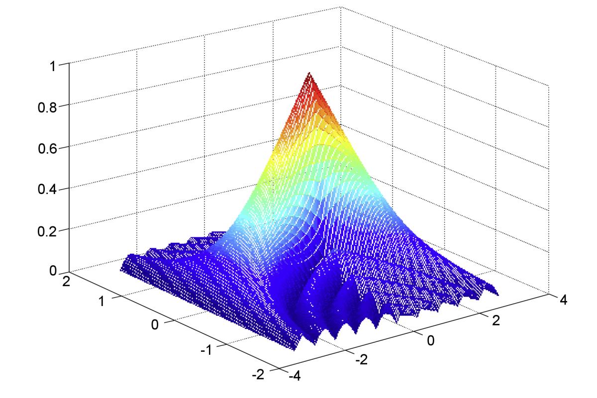
Figure 1: Ambiguity function for a rectangular pulse with a duration of 2 s (MATLAB simulation)

Figure 1: Ambiguity function for a rectangular pulse with a duration of 2 s (MATLAB simulation)
Ambiguity Function for a Rectangular Pulse
Figure 1 shows the ambiguity function as a three-dimensional surface. The two horizontal axes represent time shift and Doppler frequency. The height of the surface indicates how strongly the matched filter responds to a signal with the corresponding combination of propagation delay shift and Doppler frequency. For an exactly matching signal, the highest peak occurs at the origin. The farther the combination under consideration is from the origin, the more the filter response may change.
As an example, an unmodulated rectangular pulse is used. Its shape is particularly simple and is therefore well suited to illustrating the basic principle. The pulse duration of two seconds chosen for the simulation is for illustration only. The transmitted pulse waveform of a conventional pulsed radar using a keyed on/off modulator can be described as follows:


(5)
- TPW = transmitted pulse duration (pulse width)
- t = current time as the signal passes through the filter
When this pulse is reflected by a moving radar target, the echo signal may additionally exhibit a Doppler frequency shift. The corresponding signal is:


(6)
For this rectangular pulse, the resulting ambiguity function is:


(7)

Figure 2: Contours of the ambiguity function of an unmodulated rectangular pulse (MATLAB simulation)

Figure 2: Contours of the ambiguity function of an unmodulated rectangular pulse (MATLAB simulation)

Figure 3: Ambiguity function, cross-section along the line τ = 0

In a three-dimensional representation such as Figure 1, exact values
are difficult to read.
Therefore, two-dimensional contour plots, such as Figure 2, are also used.
The contours connect points at which the filter response has the same magnitude.
This makes it easier to see how quickly the filter response decreases when
signal propagation delay or Doppler frequency changes.
Another possibility is to examine a single cross-section through the ambiguity function. A cross-section along the line fD = 0 shows the dependence on time shift. For an unmodulated rectangular pulse, the magnitude of the filter response has a triangular shape, as is familiar from the autocorrelation of a rectangular pulse.
Figure 3, on the other hand, shows a cross-section along the line τ = 0. The time shift remains unchanged while the Doppler frequency varies. The plot shows how sensitive the matched filter is to a frequency mismatch. This illustrates why different Doppler shifts do not produce the same filter response.
Properties of the Ambiguity Function
Several general properties can be derived from the ambiguity function. For the following equations, the ambiguity function is normalized to a signal energy of 1.
- The magnitude of the normalized ambiguity function reaches its maximum value of 1 at the origin
(where τ = 0 and fᴅ = 0).
At no other point can its magnitude be greater.
This corresponds to the case in which the received signal matches the reference exactly.


- The integral of the squared magnitude of the ambiguity function remains constant
as long as the signal energy remains unchanged.
When the signal energy is normalized accordingly, the integral equals one.
This property illustrates that the distribution of the filter response
over time delay and Doppler frequency cannot be changed arbitrarily.


- The magnitude of the ambiguity function is symmetric about the origin.
Thus, a combination of positive time shift and positive Doppler frequency
has the same magnitude as the corresponding combination with both signs reversed.
However, mirror symmetry about each coordinate axis separately
does not hold for arbitrary waveforms.


For an unmodulated rectangular pulse, the ambiguity function exhibits particularly strong symmetry. Therefore, for this example, it is often sufficient to display only part of the function.
The ambiguity function thus shows how a radar waveform responds to differences in propagation delay and Doppler frequency. A narrow mainlobe in the time-delay direction helps distinguish targets at closely spaced ranges. A narrow mainlobe in the Doppler direction is important for distinguishing different Doppler frequencies. Which characteristics matter most depends on the radar system's intended task.
Further Reading:
- Nadav Levanon, Eli Mozeson: Radar Signals, Wiley-IEEE Press, 2004, ISBN 978-0-471-47378-7, Chapter 3 “Ambiguity Function”, pp. 34–52, Wiley Online Library
- Nadav Levanon: Radar Principles (Extended), lecture materials from Tel Aviv University, particularly “Matched filter” and “Ambiguity function”, Lecture slides