
Receiver Dynamic Range
begins here
limit
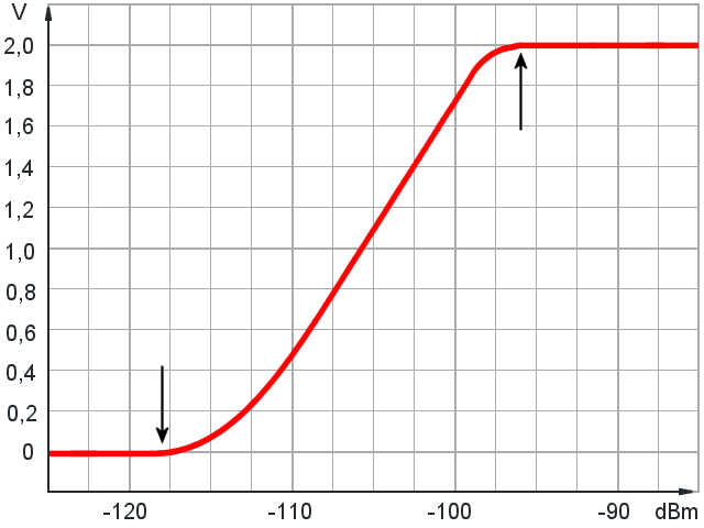
Figure 1: A receiver calibration curve showing the output signal (Y-axis) as a function of input power (X-axis). The difference between the overload point and the sensitivity limit determines the receiver dynamic range, expressed in decibels (in this example: 118 - 96 = 22 dB).

begins here
limit
Figure 1: A receiver calibration curve showing the output signal (Y-axis) as a function of input power (X-axis). The difference between the overload point and the sensitivity limit determines the receiver dynamic range, expressed in decibels (in this example: 118 - 96 = 22 dB).
Receiver Dynamic Range
The power difference between echo signals from nearby targets and those from objects at very long distances can be as much as 80 dB. Signals with such large differences in power are difficult to process. This is particularly true when the echo signals must subsequently be converted into digital data during radar signal processing.
The term “dynamic range” describes the ratio between the maximum and minimum input signal powers that a receiver can handle. For a radar receiver, the following relationship applies:
| D = | PE,max | = maximum input signal power at which the receiver has not yet entered limiting. = minimum input signal power at which the receiver still produces an output signal. | |
| PE,min |
The minimum input power PE,min is defined as 3 dB above the input noise power level. The upper limit is determined by the receiver's 1 dB compression point. At this point, the actual gain has decreased by 1 dB relative to the extrapolated linear gain characteristic. A method for directly measuring the receiver dynamic range is described in the Measurement Practice section.
If most of the radar parameters in the radar equation can be considered constant during a pulse repetition interval, the radar cross section σ and the distance to the target remain highly variable. Consequently, the minimum received power is proportional to the smallest radar cross section and inversely proportional to the fourth power of the maximum target range. Similarly, the maximum expected received power is proportional to a very large radar cross section and inversely proportional to the fourth power of the minimum measurable range.
| PE = | Ps λ2 G2 σ | = k · | σ | (2) |
| (4π)3 · R4 | R4 |
The parameters that remain constant during a pulse repetition interval are combined into a constant factor k, which cancels out in the following calculation:
| D = | PE,max | = | k · σmax / R4min | = | σmax · R4max | (3) |
| PE,min | k · σmin / R4max | σmin · R4min |
By substituting actual radar parameters into this equation, the required receiver dynamic range can be calculated for a particular radar. For example, the ASR-E uses a pulse width of 45 µs for long-range operation, resulting in a pulse-width-dependent minimum reception range of 6.75 km. The maximum range using the same transmitted pulse is specified as 60 nautical miles, or approximately 110 km. The receiver should be capable of processing echoes from targets with radar cross sections ranging from 0.1 m² (ultralight aircraft) to 100 m² (heavy transport aircraft):
| D = | 100 m² · (110 km)4 | = 7 · 107 ≈ 78.5 dB |
| 0.1 m² · (6.75 km)4 |
Thus, in addition to the weakest echo signal that can still be processed, the receiver must also be capable of handling echo signals whose power is more than 70 million times greater.
This would not be possible without certain circuit techniques that provide what is known as dynamic range compression. It is essential that this compression preserve the relative signal amplitudes: the original amplitude differences must still be recoverable mathematically during subsequent signal processing.