
Radar Range Equation
The radar range equation (or radar equation, for short) is used to describe the physical relationships from transmit power through wave propagation to reception. It can be used to determine the power Pe at the input of the radar receiver as a function of the PS PS, the range R, and the reflection properties of the object σ. Given the known sensitivity of the receiver, it is thus possible to estimate the maximum range at which, under the given conditions, the target object will generate an echo signal strong enough to be detected by the radar set. In this way, the radar equation can be used to assess the operational performance of radar sets.
Derivation of the Radar Range Equation
In the following, it is first assumed that electromagnetic waves can propagate under ideal conditions, i.e., without interference.

Figure 1: The isotropic power density is distributed over a spherical surface


Figure 1: The isotropic power density is distributed over a spherical surface
When high-frequency energy is emitted by an isotropic radiator, it is distributed uniformly in all directions. Consequently, surfaces of equal power density form spheres around the radiator. As the sphere’s radius increases, the energy is distributed over a larger area (A= 4 π R²) around the radiator. Or, to put it another way: relative to a given area, the power density S at area A decreases with increasing distance due to the radiation divergence.
Thus, the following formula applies to the omnidirectional power density Su in watts per unit area on the sphere with radius R1:


(1)
- PS = transmitted power [W]
- Su = omnidirectional power density
- R1 = distance between transmitter antenna and target [m]

Figure 2: The isotropic power density multiplied by the antenna gain yields the directional power density

Figure 2: The isotropic power density multiplied by the antenna gain yields the directional power density
If the radiation (at constant transmitted power) is limited to a partial surface of a sphere due to the directional characteristics of an antenna, this results in an increase in power density in the direction of radiation. This is referred to as antenna gain. For the directional power density Sg, the following applies:


(2)
- Sg = directional power density [W]
- Su = isotropic power density
- G = antenna gain
In reality, radar antennas are of course not “partially radiating” spherical radiators, but directional antennas (e.g., parabolic antennas or phased array antennas) with an antenna gain of 30 to 40 dB, which corresponds to a factor of 1 000 to 10 000 in the equation.
Target detection depends not only on the power density at the target’s location, but also on the limitation of how much of it is actually reflected toward the radar system. To determine the usable reflected power, the radar cross section σ is required. This quantity, which is difficult to determine, depends on several factors. It is immediately apparent that a larger surface area reflects more power than a small one; in other words:
An Airbus offers more reflective surface area than a small single-engine aircraft at the same flight attitude. Furthermore, the reflectivity strongly depends on the shape, surface texture, and the materials used.
To summarize what has been said so far, the reflected power Pr (at the target location) results from the power density Su, the antenna gain G, and the highly variable reflectivity σ : Wird das bisher gesagte zusammengefasst, so ergibt sich die reflektierte Leistung Pr (am Zielort) aus der Leistungsdichte Su, dem Antennengewinn G und der sehr variablen Rückstrahlfläche σ :
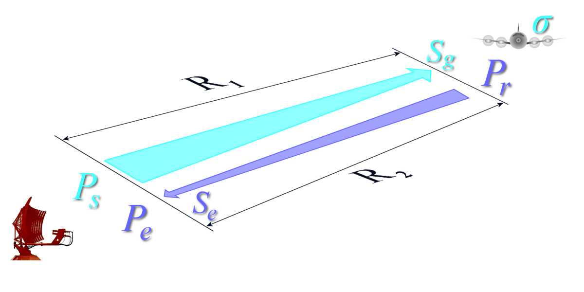
Figure 3: Relationship between equations (3) and (4)


(3)
- Pr = reflected powe [W]
- σ = Radar Cross Section (RCS) [m²]
In simplified terms, a target can in turn be regarded as a radiator based on the reflected power. The reflected power Pr then becomes the radiated power.
Since the same conditions prevail on the return path of the echoes as on the outbound path, the power density at the receiving site Se is given by:


(4)
- Se = power density at the receiving site
- Pr = reflected power [W]
- R2 = distance between target and receiving antenna [m]
At the radar antenna, the received power Pe depends on the power density Se at the receiving site and the antenna's aperture AW.
(5)
- Pe = Received power at the receiving site
- Se = Power density at the receiving site
- AW = Antenna's aperture
An effective antenna's aperture results from the fact that an antenna does not operate without losses, i.e., the geometric dimensions are not fully available as receiving area. As a rule, the effectiveness of an antenna is reduced by a factor of 0.6 to 0.7 (factor Ka) compared to what the geometric dimensions would suggest.
The following applies to the effective antenna's aperture:
(6)
- AW = effective antenna's aperture [m²]
- A = geometric dimension (area) of the antenna [m²]
- Ka = respective antenna-specific loss
This yields the power Pe at the receivers input:


So far, the forward and return paths have been considered separately in the derivations. In the next step, both paths are combined, and since the distance R1 (antenna – target) is equal to R2 (target – antenna), this is taken into account in the next step.


(9)
Another equation, which will not be derived here, relates the antenna gain G to the wavelength λ used.


(10)
Converting to the antenna face A · Ka and substituting into equation (9) yields:


(11)
After converting to the range R, the classic form of the radar equation emerges:


(12)
In deriving the radar equation, all variables that influence the undisturbed wave propagation of the radar signals were taken into account. Furthermore, the dependencies of these variables were illustrated and ultimately summarized in the classic radar equation.
Beyond this theoretical approach, the radar equation can certainly also be applied in practice, e.g., to determine the performance of radar systems. However, the form of the classical radar equation is not yet suitable for these extended considerations. Some further considerations are necessary.
With respect to a specific radar system, most parameters (Ps, G, σ) can be considered constant, as they are device parameters that vary only within small ranges. In contrast, the radar cross-section σ is a difficult-to-determine parameter and is therefore usually assumed to be the practical value of 1 m².
Under this condition, the received power Pe is of interest, which produces an echo signal that is just barely detectable in the radar receiver. This received power is called PE min. Smaller received powers are not usable, as they are lost in the noise of the receiver. Substituting PE min into the radar equation allows the equation to be used to determine the theoretical maximum range Rmax.


(13)
A practical application of this radar equation is the determination of performance data for specific radar systems with the aim of comparing and evaluating the systems.
Factors Affecting the Range of a Radar System
All considerations related to the radar equation have so far been made under the assumption that electromagnetic waves can propagate under ideal conditions. The mathematical description of the antenna gain is also based on a simplified model. In practice, however, a number of losses arise that cannot be ignored, as they can significantly reduce the effectiveness of a radar system.
To account for this, the radar equation is first extended to include the (total) loss factor Lges. Since these losses reduce the range, this factor appears in the denominator:


(14)
This factor encompasses, among other things, the types of losses listed as examples below:
- L D = internal attenuation losses along the transmit and receive paths
- L f = fluctuation losses during reflection at the target
- L Atm = atmospheric attenuation losses along the propagation path to the target and back
Internal device attenuation losses occur primarily in high-frequency components such as waveguides and filters, but also due to a radome. For a given radar system, the value of this type of loss is relatively constant and can be easily determined (measured).
Other constant factors include
atmospheric attenuation
and reflections at the Earth’s surface.
Various loss factors in the radar system
Analysis of received power
Although the magnitude of the power of the minimum detectable signal can be determined relatively easily as a comparative measurement, it is customary to break this down using a signal-to-noise ratio and the magnitude of the noise as noise power at the receiver input. An echo signal must exceed the noise level by a given signal-to-noise ratio in order to be recognized as a target sign. The limiting case is when it is equal to the noise level.
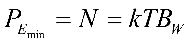

(15)
- k = 1,38·10-23 J/K, (Boltzmann constant)
- T = absolute temperature in Kelvin
- Bw = receiver bandwidth
In practice, however, at least a minimum signal-to-noise ratio is required, meaning that the echo signal should be greater than the noise itself by a factor equal to the signal-to-noise ratio. In Equation (14), PEmin is replaced by Equation (15) and the minimum signal-to-noise ratio (S/N)min is additionally inserted:
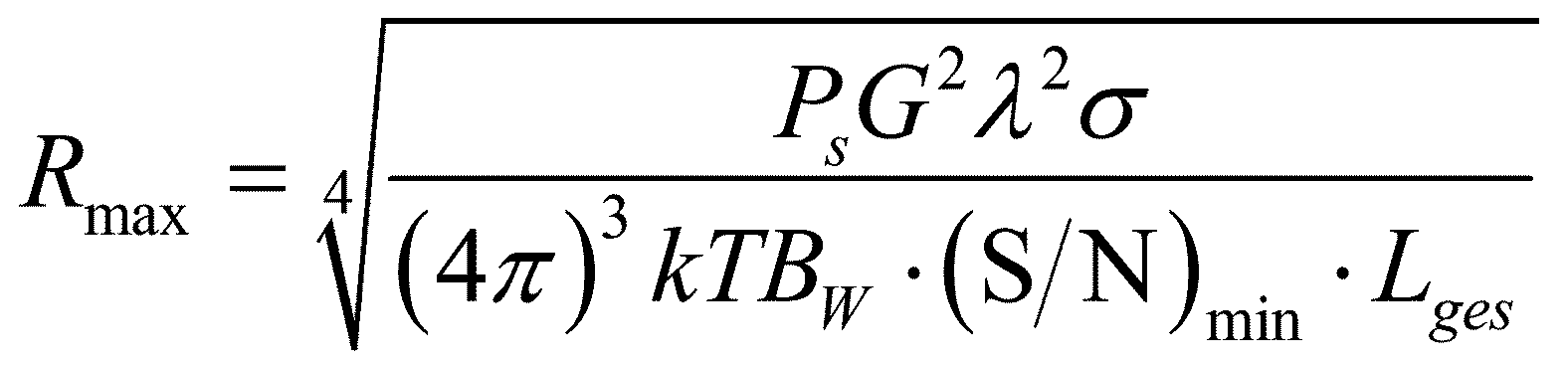
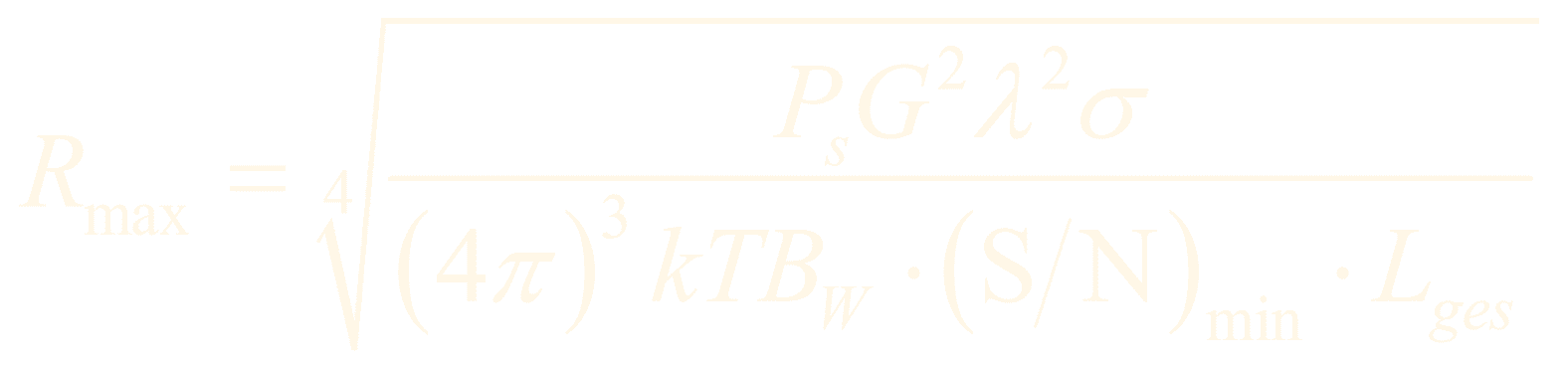
(16)
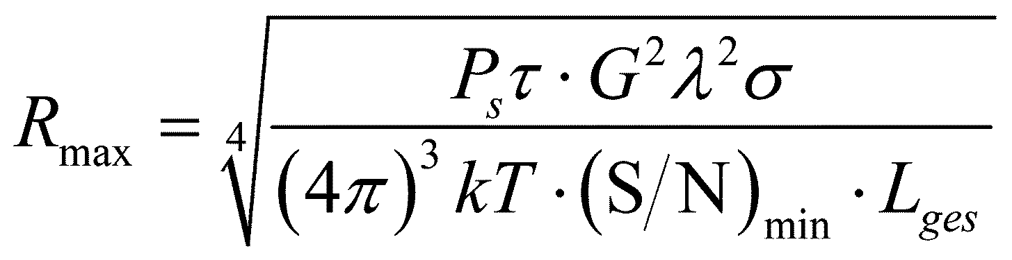
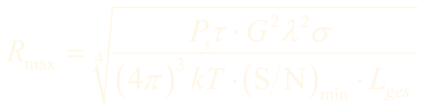
The receiver bandwidth Bw should be chosen as small as possible, but still sufficiently large to allow for low-distortion transmission of the echo pulses. In radar technology, the Rayleigh criterion is often used, which defines that the optimal bandwidth of a simple rectangular pulse is equal to the reciprocal of its duration (Bw=1/τ).
(17)
This gives us the final form of the radar equation for a pulse radar. What is interesting about this form is that the device-specific parameters (Ps·τ) correspond to an amount of energy.
For radar sets with intra-pulse modulation and pulse compression, the receiver bandwidth must be calculated based on the compressed pulse duration. One might assume that the compressed pulse duration could also be used here. However, the pulse compression ratio must then also be included in the numerator, because in pulse compression the many small sub-pulses are added coherently, but the noise is non-coherent and therefore cannot be added to the same extent.
Incidentally, multiplying the compressed transmission pulse duration by the pulse compression ratio is technically very similar to coherent pulse integration; in other words, the maximum range can also be increased using pulse integration.
Influence of the Earth's Surface

Figure 4: Multipath reception due to reflection off the Earth’s surface

Figure 4: Multipath reception due to reflection off the Earth’s surface
An extended form of the radar equation, which is no longer used today, takes additional factors into account, such as the influence of the Earth’s surface, and further breaks down the receiver sensitivity (noise factor), the coverage angle of the site (factor with sine functions), and atmospheric attenuation (factor with exponential function).


(18)
In this equation, in addition to the already known quantities:
- Kα = loss factor in place of Lges.
- Az = effective reflectivity in place of σ
- ti = pulse duration
- nR = noise figure of the receiver
- d = clarity factor of the display
- Re = initial distance of the attenuating medium
- γ = elevation angle of the target
- K = Boltzmann constant
- T0 = absolute standard temperature of 290 K
- γ = radiation angle
- δR = distance difference with increased attenuation factor
- hm = average antenna height
The fact that the formula is no longer used in this form is due to the fact that the influence of the Earth’s surface described therein is tailored to radar sets in the VHF band, which are no longer used in Europe and the USA today.
Print version of the Power-Point presentation “Understanding Radar Equation”.